SciPy - Binomial Distribution

Binomial Distribution is a discrete probability distribution and it expresses the probability of a given number of successes in a sequence of n independent experiments with a known probability of success on each trial.

The probability mass function (pmf) of binomial distribution is defined as:

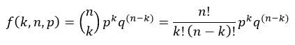
Where,

p is the probability of success in each trial
q is the probability of failure in each trial, q = 1 - p
n is number of trials
k is the number of successes which can occur anywhere among the n trials

An binomial distribution has mean np and variance npq.

The cumulative distribution function (cdf) evaluated at k, is the probability that the random variable (X) will take a value less than or equal to k. The cdf of binomial distribution is defined as:

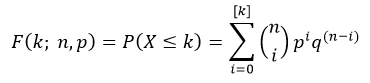
Where, [k] is the greatest integer less than or equal to k.

The scipy.stats.binom contains all the methods required to generate and work with a binomial distribution. The most frequently methods are mentioned below:

Syntax

scipy.stats.binom.pmf(k, n, p, loc=0)
scipy.stats.binom.cdf(k, n, p, loc=0)
scipy.stats.binom.ppf(q, n, p, loc=0)
scipy.stats.binom.rvs(n, p, loc=0, size=1)

Parameters

`k`	`Required.` Specify float or array_like of floats representing random variable.
`q`	`Required.` Specify float or array_like of floats representing probabilities.
`n`	`Required.` Specify number of trials, must be >= 0. Floats are also accepted, but they will be truncated to integers.
`p`	`Required.` Specify probability of success in each trial, must be in range [0, 1]. float or array_like of floats.
`loc`	`Optional.` Specify the location of the distribution. Default is 0.
`size`	`Optional.` Specify output shape.

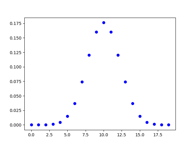
binom.pmf()

The binom.pmf() function measures probability mass function (pmf) of the distribution.

from scipy.stats import binom
import matplotlib.pyplot as plt
import numpy as np

#creating an array of values between
#0 to 20 with a difference of 1
x = np.arange(0, 20, 1)
   
y = binom.pmf(x, 20, 0.5)
   
plt.plot(x, y, 'bo') 
plt.show()

The output of the above code will be:

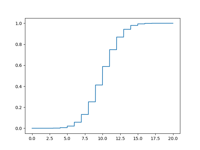
binom.cdf()

The binom.cdf() function returns cumulative distribution function (cdf) of the distribution.

from scipy.stats import binom
import matplotlib.pyplot as plt
import numpy as np

#creating an array of values between
#0 to 20 with a difference of 0.01
x = np.arange(0, 20, 0.01)
   
y = binom.cdf(x, 20, 0.5)
   
plt.plot(x, y) 
plt.show()

The output of the above code will be:

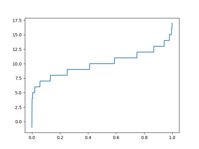
binom.ppf()

The binom.ppf() function takes the probability value and returns cumulative value corresponding to probability value of the distribution.

from scipy.stats import binom
import matplotlib.pyplot as plt
import numpy as np

#creating an array of probability from
#0 to 1 with a difference of 0.001
x = np.arange(0, 1, 0.001)
   
y = binom.ppf(x, 20, 0.5)
   
plt.plot(x, y) 
plt.show()

The output of the above code will be:

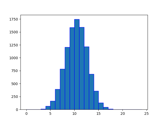
binom.rvs()

The binom.ppf() function generates an array containing specified number of random values drawn from the given binomial distribution. In the example below, a histogram is plotted to visualize the result.

from scipy.stats import binom
import matplotlib.pyplot as plt
import numpy as np

#fixing the seed for reproducibility
#of the result
np.random.seed(10)

#creating a vector containing 10000
#random values from binomial distribution
y = binom.rvs(20, 0.5, 0, 10000)

#creating bin
bin = np.arange(0,25,1)  

plt.hist(y, bins=bin, edgecolor='blue') 
plt.show()

The output of the above code will be: