SciPy - Geometric Distribution

Geometric Distribution is a discrete probability distribution and it expresses the probability distribution of the random variable (X) representing number of Bernoulli trials needed to get one success.

The probability mass function (pmf) of geometric distribution is defined as:

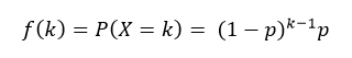
Where, k is the number of Bernoulli trials (k = 1,2...) and p is probability of success in each trial.

An geometric distribution has mean 1/p and variance (1-p)/p².

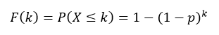
The cumulative distribution function (cdf) evaluated at k, is the probability that the random variable (X) will take a value less than or equal to k. The cdf of geometric distribution is defined as:

The scipy.stats.geom contains all the methods required to generate and work with a geometric distribution. The most frequently methods are mentioned below:

Syntax

scipy.stats.geom.pmf(k, p, loc=0)
scipy.stats.geom.cdf(k, p, loc=0)
scipy.stats.geom.ppf(q, p, loc=0)
scipy.stats.geom.rvs(p, loc=0, size=1)

Parameters

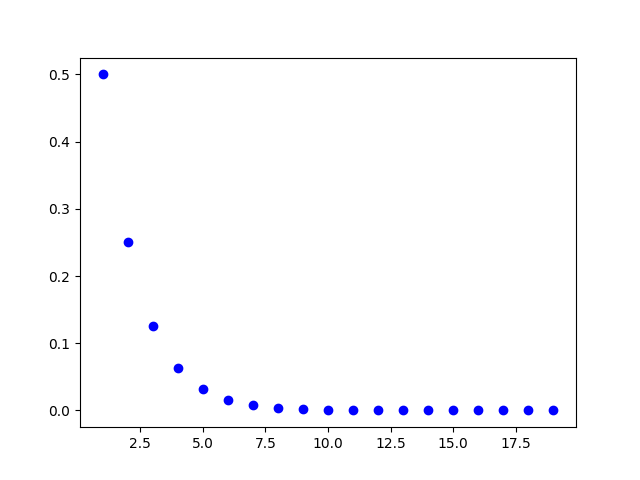
geom.pmf()

The geom.pmf() function measures probability mass function (pmf) of the distribution.

from scipy.stats import geom
import matplotlib.pyplot as plt
import numpy as np

#creating an array of values between
#1 to 20 with a difference of 1
x = np.arange(1, 20, 1)
   
y = geom.pmf(x, 0.5)
   
plt.plot(x, y, 'bo') 
plt.show()

The output of the above code will be:

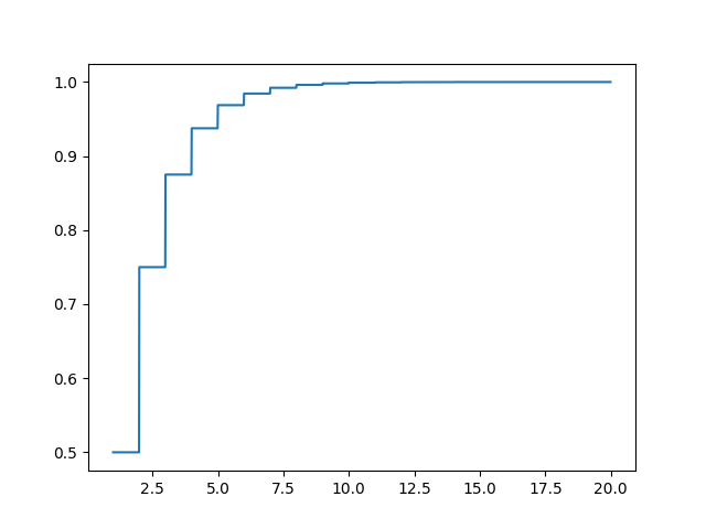
geom.cdf()

The geom.cdf() function returns cumulative distribution function (cdf) of the distribution.

from scipy.stats import geom
import matplotlib.pyplot as plt
import numpy as np

#creating an array of values between
#1 to 20 with a difference of 0.01
x = np.arange(1, 20, 0.01)
   
y = geom.cdf(x, 0.5)
   
plt.plot(x, y) 
plt.show()

The output of the above code will be:

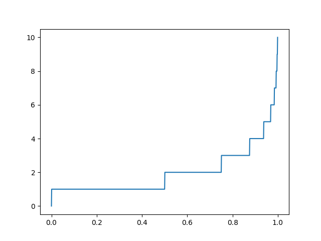
geom.ppf()

The geom.ppf() function takes the probability value and returns cumulative value corresponding to probability value of the distribution.

from scipy.stats import geom
import matplotlib.pyplot as plt
import numpy as np

#creating an array of probability from
#0 to 1 with a difference of 0.001
x = np.arange(0, 1, 0.001)
   
y = geom.ppf(x, 0.5)
   
plt.plot(x, y) 
plt.show()

The output of the above code will be:

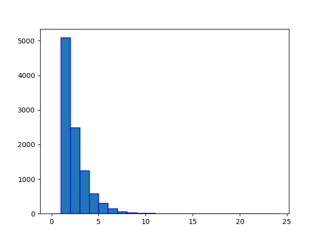
geom.rvs()

The geom.ppf() function generates an array containing specified number of random values drawn from the given geometric distribution. In the example below, a histogram is plotted to visualize the result.

from scipy.stats import geom
import matplotlib.pyplot as plt
import numpy as np

#fixing the seed for reproducibility
#of the result
np.random.seed(10)

#creating a vector containing 10000
#random values from geometric distribution
y = geom.rvs(0.5, 0, 10000)

#creating bin
bin = np.arange(0,25,1)  

plt.hist(y, bins=bin, edgecolor='blue') 
plt.show()

The output of the above code will be: