NumPy - Binomial Distribution

Binomial Distribution is a discrete probability distribution and it expresses the probability of a given number of successes in a sequence of n independent experiments with a known probability of success on each trial.

The probability mass function (pmf) of binomial distribution is defined as:

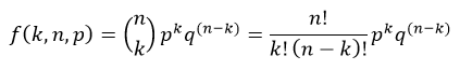
Where,

• p is the probability of success in each trial
• q is the probability of failure in each trial, q = 1 - p
• n is number of trials
• k is the number of successes which can occur anywhere among the n trials

An binomial distribution has mean np and variance npq.

The cumulative distribution function (cdf) evaluated at k, is the probability that the random variable (X) will take a value less than or equal to k. The cdf of binomial distribution is defined as:

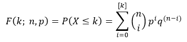
Where, [k] is the greatest integer less than or equal to k.

The NumPy random.binomial() function returns random samples from a binomial distribution.

Syntax

numpy.random.binomial(n, p, size=None)

Parameters

Return Value

Returns samples from the parameterized binomial distribution. ndarray or scalar.

Example: Values from binomial distribution

In the example below, random.binomial() function is used to create a matrix of given shape containing random values drawn from specified binomial distribution.

import numpy as np

size = (5,3)

sample = np.random.binomial(20, 0.5, size)
print(sample)

The possible output of the above code could be:

[[ 8  8 10]
 [ 5  9  8]
 [11  9 12]
 [12  7 11]
 [ 9  9 10]]

Plotting binomial distribution

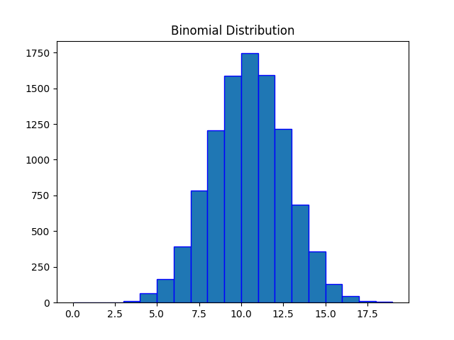
Example: Histogram plot

Matplotlib is a plotting library for the Python which can be used to plot the probability mass function (pmf) of binomial distribution using hist() function.

import matplotlib.pyplot as plt
import numpy as np

#fixing the seed for reproducibility
#of the result
np.random.seed(10)

size = 10000
#drawing 10000 sample from 
#binomial distribution
sample = np.random.binomial(20, 0.5, size)
bin = np.arange(0,20,1)

plt.hist(sample, bins=bin, edgecolor='blue') 
plt.title("Binomial Distribution") 
plt.show()

The output of the above code will be:

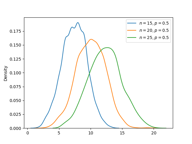
Example: Comparing pmfs

Multiple mass functions can be compared graphically using Seaborn kdeplot() function. In the example below, pmf of three binomial distributions (each with different number of trials but same probability of success) are compared.

import numpy as np
import matplotlib.pyplot as plt
import seaborn as sns

#fixing the seed for reproducibility
#of the result
np.random.seed(10)

size = 1000
#plotting 1000 sample from 
#different binomial distribution
sns.kdeplot(np.random.binomial(15, 0.5, size))
sns.kdeplot(np.random.binomial(20, 0.5, size))
sns.kdeplot(np.random.binomial(25, 0.5, size))

plt.legend(["$n = 15, p = 0.5$", 
            "$n = 20, p = 0.5$", 
            "$n = 25, p = 0.5$"])
plt.show()

The output of the above code will be:

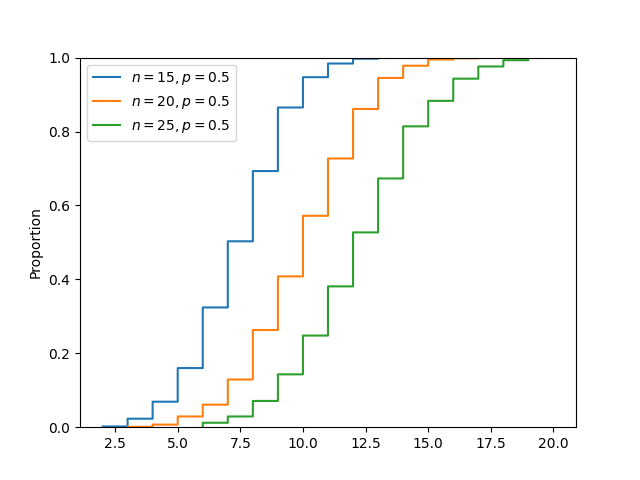
Example: Comparing cdfs

Multiple cumulative distribution functions can be compared graphically using Seaborn ecdfplot() function. In the example below, cdf of three binomial distributions (each with different number of trials but same probability of success) are compared.

import numpy as np
import matplotlib.pyplot as plt
import seaborn as sns

#fixing the seed for reproducibility
#of the result
np.random.seed(10)

size = 1000
#plotting 1000 sample from 
#different binomial distribution
sns.ecdfplot(np.random.binomial(15, 0.5, size))
sns.ecdfplot(np.random.binomial(20, 0.5, size))
sns.ecdfplot(np.random.binomial(25, 0.5, size))

plt.legend(["$n = 15, p = 0.5$", 
            "$n = 20, p = 0.5$", 
            "$n = 25, p = 0.5$"])
plt.show()

The output of the above code will be: