NumPy - Exponential Distribution

Exponential distribution is the probability distribution of the time between events in a Poisson point process, i.e., a process in which events occur continuously and independently at a constant average rate. It is a particular case of the gamma distribution. For example, customers arriving at a store, file requests on a server etc.

The probability density function (pdf) of exponential distribution is defined as:

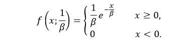
Where, β is the scale parameter which is the inverse of the rate parameter λ = 1/β.

An exponential distribution has mean β and variance β².

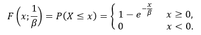
The cumulative distribution function (cdf) evaluated at x, is the probability that the random variable (X) will take a value less than or equal to x. The cdf of exponential distribution is defined as:

The NumPy random.exponential() function returns random samples from a exponential distribution.

Syntax

numpy.random.exponential(scale=1.0, size=None)

Parameters

Return Value

Returns samples from the parameterized exponential distribution. ndarray or scalar.

Example: Values from exponential distribution

In the example below, random.exponential() function is used to create a matrix of given shape containing random values drawn from specified exponential distribution.

import numpy as np

size = (5,3)

sample = np.random.exponential(1, size)
print(sample)

The possible output of the above code could be:

[[0.71318134 0.51261985 2.21255627]
 [0.38593481 0.54545811 0.39075276]
 [0.56583485 1.59475025 0.13879821]
 [0.82487244 0.20735562 1.33014896]
 [0.21085364 1.06640552 1.33323175]]

Plotting exponential distribution

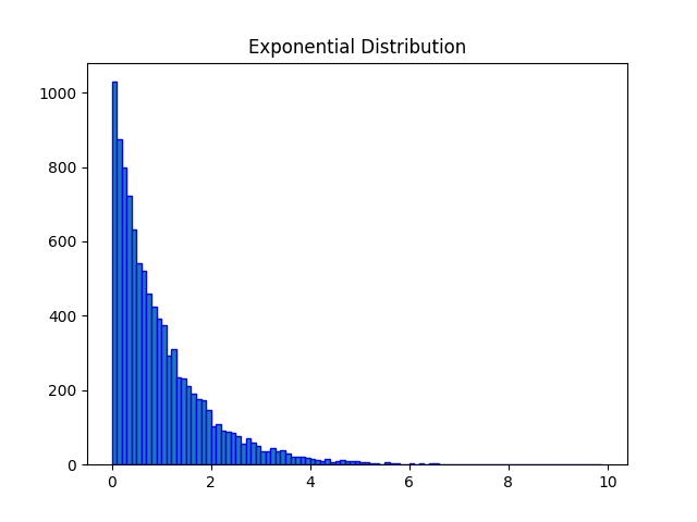
Example: Density plot

Matplotlib is a plotting library for the Python which can be used to plot the probability density function (pdf) of exponential distribution using hist() function.

import matplotlib.pyplot as plt
import numpy as np

#fixing the seed for reproducibility
#of the result
np.random.seed(10)

size = 10000
#drawing 10000 sample from 
#exponential distribution
sample = np.random.exponential(1, size)
bin = np.arange(0,10,0.1)

plt.hist(sample, bins=bin, edgecolor='blue') 
plt.title("Exponential Distribution") 
plt.show()

The output of the above code will be:

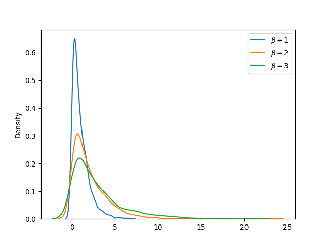
Example: Comparing pdfs

Multiple probability density functions can be compared graphically using Seaborn kdeplot() function. In the example below, pdf of three exponential distributions (with scale factor 1, 2 and 3 respectively) are compared.

import numpy as np
import matplotlib.pyplot as plt
import seaborn as sns

#fixing the seed for reproducibility
#of the result
np.random.seed(10)

size = 1000
#plotting 1000 sample from 
#different exponential distribution
sns.kdeplot(np.random.exponential(1, size))
sns.kdeplot(np.random.exponential(2, size))
sns.kdeplot(np.random.exponential(3, size))

plt.legend([r"$\beta = 1$", 
            r"$\beta = 2$", 
            r"$\beta = 3$"])
plt.show()

The output of the above code will be:

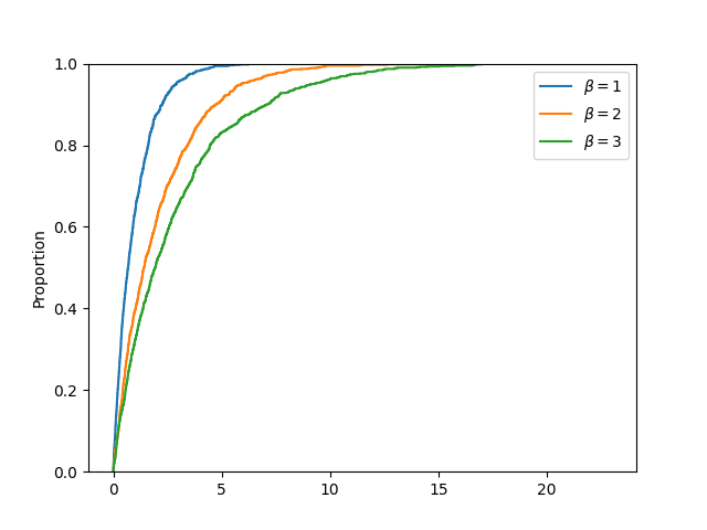
Example: Comparing cdfs

Multiple cumulative distribution functions can be compared graphically using Seaborn ecdfplot() function. In the example below, cdf of three exponential distributions (with scale factor 1, 2 and 3 respectively) are compared.

import numpy as np
import matplotlib.pyplot as plt
import seaborn as sns

#fixing the seed for reproducibility
#of the result
np.random.seed(10)

size = 1000
#plotting 1000 sample from 
#different exponential distribution
sns.ecdfplot(np.random.exponential(1, size))
sns.ecdfplot(np.random.exponential(2, size))
sns.ecdfplot(np.random.exponential(3, size))

plt.legend([r"$\beta = 1$", 
            r"$\beta = 2$", 
            r"$\beta = 3$"])
plt.show()

The output of the above code will be: