NumPy - Logistic Distribution

Logistic distribution is a continuous probability distribution. Its cumulative distribution function is the logistic function, which appears in logistic regression and feedforward neural networks. It resembles the logistic distribution in shape but has heavier tails.

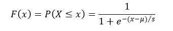
The probability density function (pdf) of logistic distribution is defined as:

Where, μ is the mean or expectation of the distribution and s is the scale parameter of the distribution.

An exponential distribution has mean μ and variance s²𝜋²/3.

The cumulative distribution function (cdf) evaluated at x, is the probability that the random variable (X) will take a value less than or equal to x. The cdf of logistic distribution is defined as:

The NumPy random.logistic() function returns random samples from a logistic distribution.

Syntax

numpy.random.logistic(loc=0.0, scale=1.0, size=None)

Parameters

Return Value

Returns samples from the parameterized logistic distribution. ndarray or scalar.

Example: Values from logistic distribution

In the example below, random.logistic() function is used to create a matrix of given shape containing random values drawn from specified logistic distribution.

import numpy as np

size = (5,3)

sample = np.random.logistic(0, 1, size)
print(sample)

The possible output of the above code could be:

[[-1.11416732 -0.69983364 -0.28651865]
 [-3.05668874 -1.35517427 -3.50476354]
 [ 0.78448327  0.2499033  -0.36716532]
 [-0.45759849 -1.3434462   0.8690071 ]
 [-0.74228078  1.08577009 -2.35079969]]

Plotting logistic distribution

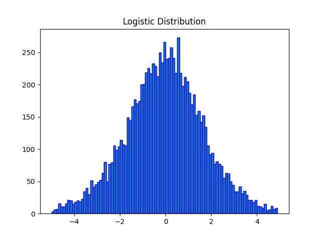
Example: Density plot

Matplotlib is a plotting library for the Python which can be used to plot the probability density function (pdf) of logistic distribution using hist() function.

import matplotlib.pyplot as plt
import numpy as np

#fixing the seed for reproducibility
#of the result
np.random.seed(10)

size = 10000
#drawing 10000 sample from 
#logistic distribution
sample = np.random.logistic(0, 1, size)
bin = np.arange(-5,5,0.1)

plt.hist(sample, bins=bin, edgecolor='blue') 
plt.title("Logistic Distribution") 
plt.show()

The output of the above code will be:

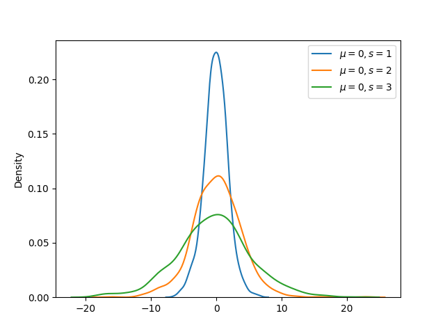
Example: Comparing pdfs

Multiple probability density functions can be compared graphically using Seaborn kdeplot() function. In the example below, pdf of three logistic distributions (each with mean 0 and scale parameter 1, 2 and 3 respectively) are compared.

import numpy as np
import matplotlib.pyplot as plt
import seaborn as sns

#fixing the seed for reproducibility
#of the result
np.random.seed(10)

size = 1000
#plotting 1000 sample from 
#different logistic distribution
sns.kdeplot(np.random.logistic(0, 1, size))
sns.kdeplot(np.random.logistic(0, 2, size))
sns.kdeplot(np.random.logistic(0, 3, size))

plt.legend([r"$\mu = 0, s = 1$", 
            r"$\mu = 0, s = 2$", 
            r"$\mu = 0, s = 3$"])
plt.show()

The output of the above code will be:

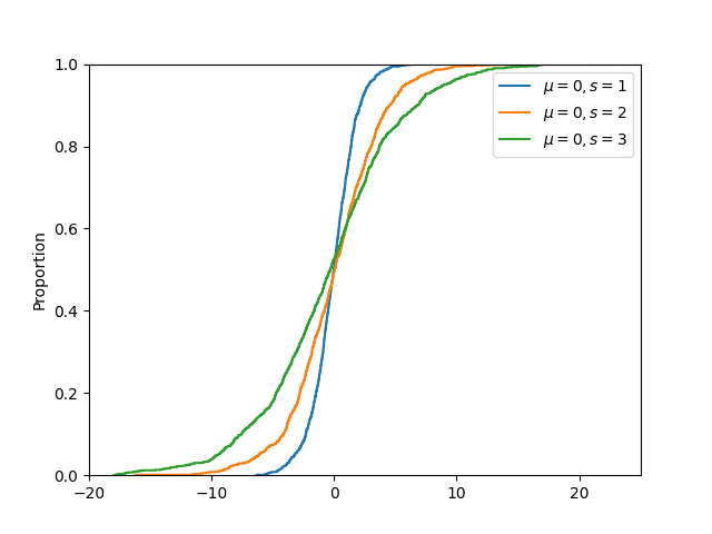
Example: Comparing cdfs

Multiple cumulative distribution functions can be compared graphically using Seaborn ecdfplot() function. In the example below, cdf of three logistic distributions (each with mean 0 and scale parameter 1, 2 and 3 respectively) are compared.

import numpy as np
import matplotlib.pyplot as plt
import seaborn as sns

#fixing the seed for reproducibility
#of the result
np.random.seed(10)

size = 1000
#plotting 1000 sample from 
#different logistic distribution
sns.ecdfplot(np.random.logistic(0, 1, size))
sns.ecdfplot(np.random.logistic(0, 2, size))
sns.ecdfplot(np.random.logistic(0, 3, size))

plt.legend([r"$\mu = 0, s = 1$", 
            r"$\mu = 0, s = 2$", 
            r"$\mu = 0, s = 3$"])
plt.show()

The output of the above code will be:

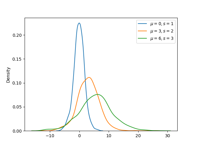
Example: comparing pdfs (different mean and scale parameter)

In the example below, three logistic distributions each with different mean and scale parameters are graphically compared.

import numpy as np
import matplotlib.pyplot as plt
import seaborn as sns

#fixing the seed for reproducibility
#of the result
np.random.seed(10)

size = 1000
#plotting 1000 sample from 
#different logistic distribution
sns.kdeplot(np.random.logistic(0, 1, size))
sns.kdeplot(np.random.logistic(3, 2, size))
sns.kdeplot(np.random.logistic(6, 3, size))

plt.legend([r"$\mu = 0, s = 1$", 
            r"$\mu = 3, s = 2$", 
            r"$\mu = 6, s = 3$"])
plt.show()

The output of the above code will be: