NumPy - Poisson Distribution

Poisson Distribution is a discrete probability distribution and it expresses the probability of a given number of events occurring in a fixed interval of time or space if these events occur with a known constant mean rate and independently of the time since the last event.

The probability mass function (pmf) of poisson distribution is defined as:

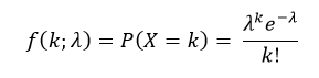
Where, k is the number of occurrences (k=0,1,2...), λ is average number of events.

An poisson distribution has mean λ and variance λ.

The cumulative distribution function (cdf) evaluated at k, is the probability that the random variable (X) will take a value less than or equal to k. The cdf of poisson distribution is defined as:

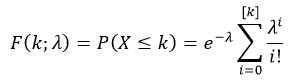
Where, [k] is the greatest integer less than or equal to k.

The NumPy random.poisson() function returns random samples from a poisson distribution.

Syntax

numpy.random.poisson(lam=1.0, size=None)

Parameters

Return Value

Returns samples from the parameterized poisson distribution. ndarray or scalar.

Example: Values from poisson distribution

In the example below, random.poisson() function is used to create a matrix of given shape containing random values drawn from specified poisson distribution.

import numpy as np

size = (5,3)

sample = np.random.poisson(10, size)
print(sample)

The possible output of the above code could be:

[[13 10  9]
 [11 11 10]
 [15 12 11]
 [ 6 12 10]
 [12 10 11]]

Plotting poisson distribution

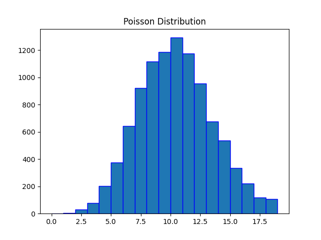
Example: Histogram plot

Matplotlib is a plotting library for the Python which can be used to plot the probability mass function (pmf) of poisson distribution using hist() function.

import matplotlib.pyplot as plt
import numpy as np

#fixing the seed for reproducibility
#of the result
np.random.seed(10)

size = 10000
#drawing 10000 sample from 
#poisson distribution
sample = np.random.poisson(10, size)
bin = np.arange(0,20,1)

plt.hist(sample, bins=bin, edgecolor='blue') 
plt.title("Poisson Distribution") 
plt.show()

The output of the above code will be:

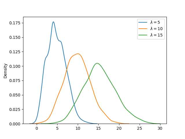
Example: Comparing pmfs

Multiple mass functions can be compared graphically using Seaborn kdeplot() function. In the example below, pmf of three poisson distributions (each with different λ) are compared.

import numpy as np
import matplotlib.pyplot as plt
import seaborn as sns

#fixing the seed for reproducibility
#of the result
np.random.seed(10)

size = 1000
#plotting 1000 sample from 
#different poisson distribution
sns.kdeplot(np.random.poisson(5, size))
sns.kdeplot(np.random.poisson(10, size))
sns.kdeplot(np.random.poisson(15, size))

plt.legend([r"$\lambda = 5$", 
            r"$\lambda = 10$", 
            r"$\lambda = 15$"])
plt.show()

The output of the above code will be:

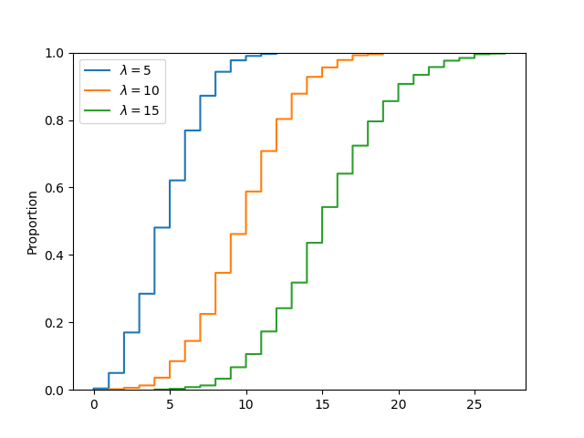
Example: Comparing cdfs

Multiple cumulative distribution functions can be compared graphically using Seaborn ecdfplot() function. In the example below, cdf of three poisson distributions (each with different λ) are compared.

import numpy as np
import matplotlib.pyplot as plt
import seaborn as sns

#fixing the seed for reproducibility
#of the result
np.random.seed(10)

size = 1000
#plotting 1000 sample from 
#different poisson distribution
sns.ecdfplot(np.random.poisson(5, size))
sns.ecdfplot(np.random.poisson(10, size))
sns.ecdfplot(np.random.poisson(15, size))

plt.legend([r"$\lambda = 5$", 
            r"$\lambda = 10$", 
            r"$\lambda = 15$"])
plt.show()

The output of the above code will be: