R - Binomial Distribution

Binomial Distribution is a discrete probability distribution and it expresses the probability of a given number of successes in a sequence of n independent experiments with a known probability of success on each trial.

The probability mass function (pmf) of binomial distribution is defined as:

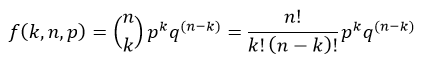
Where,

• p is the probability of success in each trial
• q is the probability of failure in each trial, q = 1 - p
• n is number of trials
• k is the number of successes which can occur anywhere among the n trials

An binomial distribution has mean np and variance npq.

The cumulative distribution function (cdf) evaluated at k, is the probability that the random variable (X) will take a value less than or equal to k. The cdf of binomial distribution is defined as:

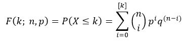
Where, [k] is the greatest integer less than or equal to k.

In R, there are four functions which can be used to generate binomial distribution.

Syntax

dbinom(x, size, prob)
pbinom(q, size, prob)
qbinom(p, size, prob)
rbinom(n, size, prob)

Parameters

dbinom()

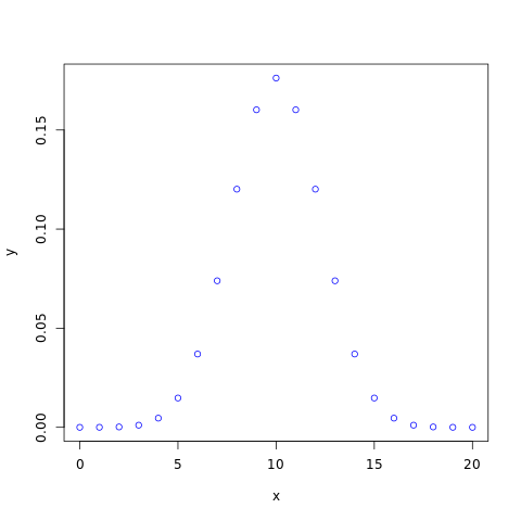
The dbinom() function measures probability mass function (pmf) of the distribution.

#creating a sequence of values between
#0 to 20 with a difference of 1
x <- seq(0, 20, by=1)
   
y <- dbinom(x, 20, 0.5)
   
#naming the file
png(file = "binomial.png")

#plotting the graph
plot(x, y, col="blue")

#saving the file
dev.off()

The output of the above code will be:

pbinom()

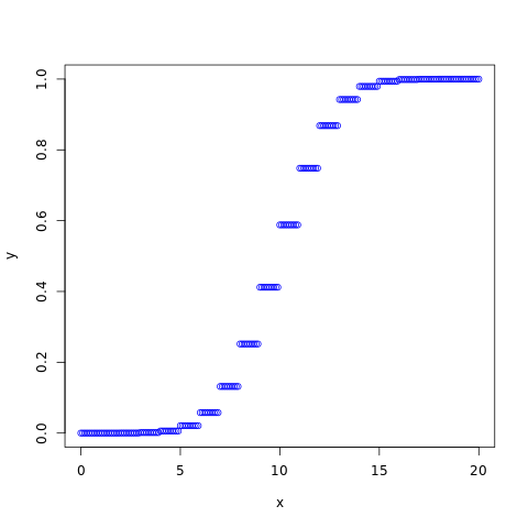
The pbinom() function returns cumulative distribution function (cdf) of the distribution.

#creating a sequence of values between
#0 to 20 with a difference of 0.1
x <- seq(0, 20, by=0.1)
   
y <- pbinom(x, 20, 0.5)
   
#naming the file
png(file = "binomial.png")

#plotting the graph
plot(x, y, col="blue")

#saving the file
dev.off()

The output of the above code will be:

qbinom()

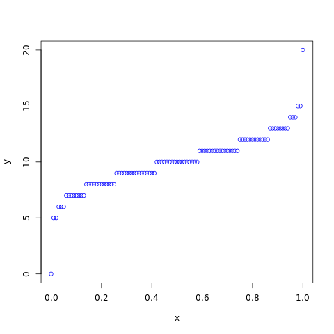
The qbinom() function takes the probability value and returns cumulative value corresponding to probability value of the distribution.

#creating a sequence of probability from
#0 to 1 with a difference of 0.01
x <- seq(0, 1, by=0.01)
   
y <- qbinom(x, 20, 0.5)
   
#naming the file
png(file = "binomial.png")

#plotting the graph
plot(x, y, col="blue")

#saving the file
dev.off()

The output of the above code will be:

rbinom()

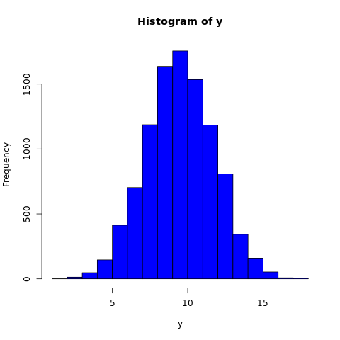
The rbinom() function generates a vector containing specified number of random values from the given binomial distribution. In the example below, a histogram is plotted to visualize the result.

#fixing the seed to maintain the
#reproducibility of the result
set.seed(10)
x <- 10000

#creating a vector containing 10000 random
#values from the given binomial distribution
y <- rbinom(x, 20, 0.5)
   
#naming the file
png(file = "binomial.png")

#plotting the graph
hist(y, col="blue")

#saving the file
dev.off()

The output of the above code will be: