R - Weibull Distribution

Weibull Distribution is a continuous probability distribution and it is widely used analyze life data, model failure times and access product reliability. It can also fit a huge range of data from many other fields like economics, hydrology, biology, engineering sciences.

The probability density function (pdf) of weibull distribution is defined as:

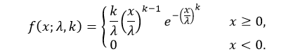
Where, k > 0 is the shape parameter and λ > 0 is the scale parameter of the distribution.

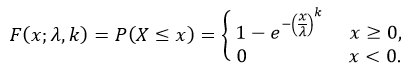
The cumulative distribution function (cdf) evaluated at x, is the probability that the random variable (X) will take a value less than or equal to x. The cdf of weibull distribution is defined as:

In R, there are four functions which can be used to generate weibull distribution.

Syntax

dweibull(x, shape, scale)
pweibull(q, shape, scale)
qweibull(p, shape, scale)
rweibull(n, shape, scale)

Parameters

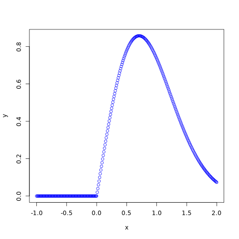
dweibull()

The dweibull() function measures probability density function (pdf) of the distribution.

#creating a sequence of values between
#-1 to 2 with a difference of 0.01
x <- seq(-1, 2, by=0.01)
   
y <- dweibull(x, 2, 1)
   
#naming the file
png(file = "weibull.png")

#plotting the graph
plot(x, y, col="blue")

#saving the file
dev.off()

The output of the above code will be:

pweibull()

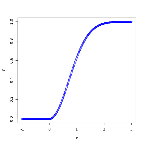
The pweibull() function returns cumulative distribution function (cdf) of the distribution.

#creating a sequence of values between
#-1 to 3 with a difference of 0.01
x <- seq(-1, 3, by=0.01)
   
y <- pweibull(x, 2, 1)
   
#naming the file
png(file = "weibull.png")

#plotting the graph
plot(x, y, col="blue")

#saving the file
dev.off()

The output of the above code will be:

qweibull()

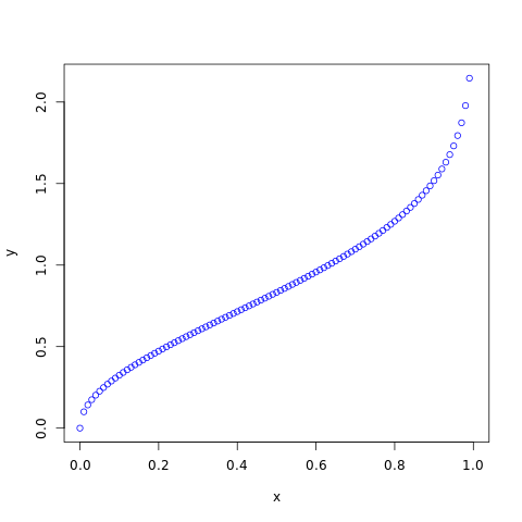
The qweibull() function takes the probability value and returns cumulative value corresponding to probability value of the distribution.

#creating a sequence of probability from
#0 to 1 with a difference of 0.01
x <- seq(0, 1, by=0.01)
   
y <- qweibull(x, 2, 1)
   
#naming the file
png(file = "weibull.png")

#plotting the graph
plot(x, y, col="blue")

#saving the file
dev.off()

The output of the above code will be:

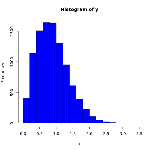
rweibull()

The rweibull() function generates a vector containing specified number of random numbers from the specified weibull distribution. In the example below, a histogram is plotted to visualize the result.

#fixing the seed to maintain the
#reproducibility of the result
set.seed(10)
x <- 10000

#creating a vector containing 10000 random
#values from the given weibull distribution
y <- rweibull(x, 2, 1)
   
#naming the file
png(file = "weibull.png")

#plotting the graph
hist(y, col="blue")

#saving the file
dev.off()

The output of the above code will be: