R - Logistic Distribution

Logistic distribution is a continuous probability distribution. Its cumulative distribution function is the logistic function, which appears in logistic regression and feedforward neural networks. It resembles the logistic distribution in shape but has heavier tails.

The probability density function (pdf) of logistic distribution is defined as:

Where, μ is the mean or expectation of the distribution and s is the scale parameter of the distribution.

An exponential distribution has mean μ and variance s²𝜋²/3.

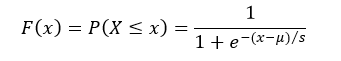
The cumulative distribution function (cdf) evaluated at x, is the probability that the random variable (X) will take a value less than or equal to x. The cdf of logistic distribution is defined as:

In R, there are four functions which can be used to generate logistic distribution.

Syntax

dlogis(x, location, scale)
plogis(q, location, scale)
qlogis(p, location, scale)
rlogis(n, location, scale)

Parameters

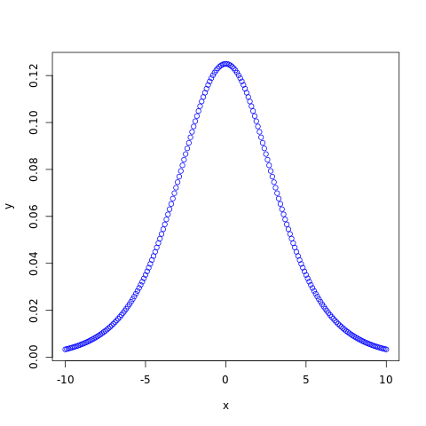
dlogis()

The dlogis() function measures probability density function (pdf) of the distribution.

#creating a sequence of values between
#-10 to 10 with a difference of 0.1
x <- seq(-10, 10, by=0.1)
   
y <- dlogis(x, 0, 2)
   
#naming the file
png(file = "logistic.png")

#plotting the graph
plot(x, y, col="blue")

#saving the file
dev.off()

The output of the above code will be:

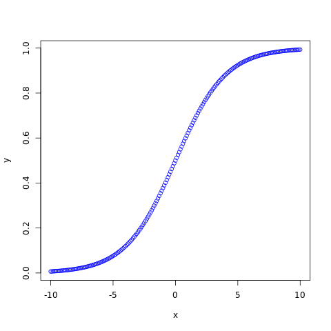
plogis()

The plogis() function returns cumulative distribution function (cdf) of the distribution.

#creating a sequence of values between
#-10 to 10 with a difference of 0.1
x <- seq(-10, 10, by=0.1)
   
y <- plogis(x, 0, 2)
   
#naming the file
png(file = "logistic.png")

#plotting the graph
plot(x, y, col="blue")

#saving the file
dev.off()

The output of the above code will be:

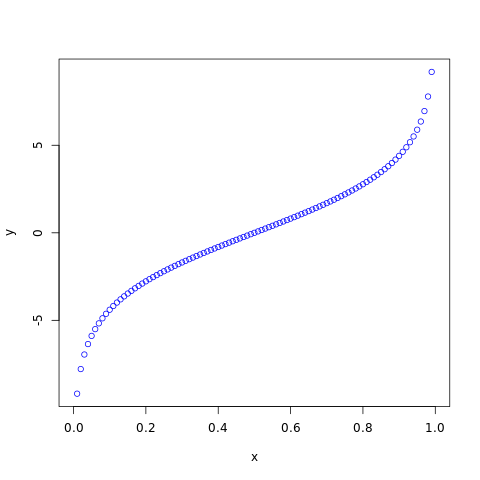
qlogis()

The qlogis() function takes the probability value and returns cumulative value corresponding to probability value of the distribution.

#creating a sequence of probability from
#0 to 1 with a difference of 0.01
x <- seq(0, 1, by=0.01)
   
y <- qlogis(x, 0, 2)
   
#naming the file
png(file = "logistic.png")

#plotting the graph
plot(x, y, col="blue")

#saving the file
dev.off()

The output of the above code will be:

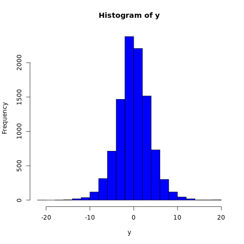
rlogis()

The rlogis() function generates a vector containing specified number of random values from the given logistic distribution. In the example below, a histogram is plotted to visualize the result.

#fixing the seed to maintain the
#reproducibility of the result
set.seed(10)
x <- 10000

#creating a vector containing 10000
#logistically distributed random values  
y <- rlogis(x, 0, 2)
   
#naming the file
png(file = "logistic.png")

#plotting the graph
hist(y, col="blue")

#saving the file
dev.off()

The output of the above code will be: