R - Normal Distribution

Normal (Gaussian) Distribution is a probability function that describes how the values of a variable are distributed. It is a symmetric distribution about its mean where most of the observations cluster around the mean and the probabilities for values further away from the mean taper off equally in both directions. It is the most important probability distribution function used in statistics because of its advantages in real case scenarios. For example, the height of the population, measurement errors etc.

The probability density function (pdf) of normal distribution is defined as:

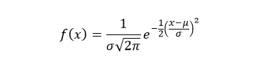
Where, μ is the mean or expectation of the distribution and σ is the standard deviation of the distribution.

An normal distribution has mean μ and variance σ². A normal distribution with μ=0 and σ=1 is called standard normal distribution.

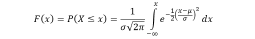
The cumulative distribution function (cdf) evaluated at x, is the probability that the random variable (X) will take a value less than or equal to x. The cdf of normal distribution is defined as:

In R, there are four functions which can be used to generate normal distribution.

Syntax

dnorm(x, mean, sd)
pnorm(q, mean, sd)
qnorm(p, mean, sd)
rnorm(n, mean, sd)

Parameters

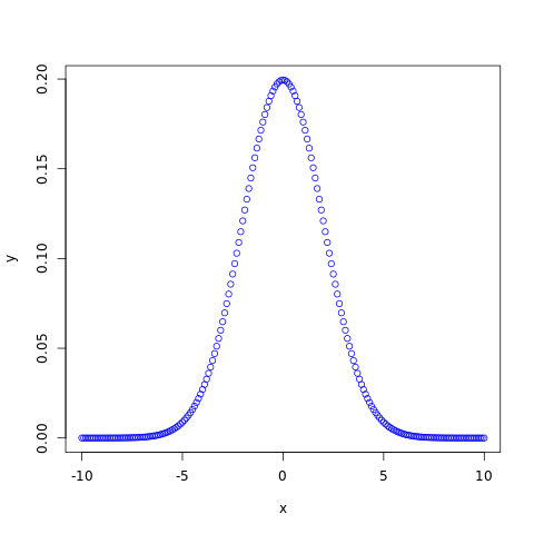
dnorm()

The dnorm() function measures probability density function (pdf) of the distribution.

#creating a sequence of values between
#-10 to 10 with a difference of 0.1
x <- seq(-10, 10, by=0.1)
   
y <- dnorm(x, 0, 2)
   
#naming the file
png(file = "normal.png")

#plotting the graph
plot(x, y, col="blue")

#saving the file
dev.off()

The output of the above code will be:

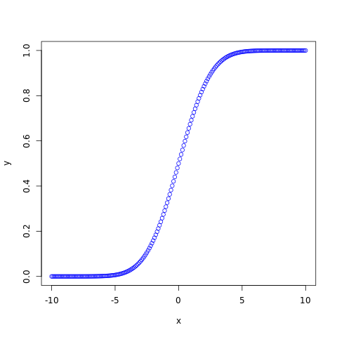
pnorm()

The pnorm() function returns cumulative distribution function (cdf) of the distribution.

#creating a sequence of values between
#-10 to 10 with a difference of 0.1
x <- seq(-10, 10, by=0.1)
   
y <- pnorm(x, 0, 2)
   
#naming the file
png(file = "normal.png")

#plotting the graph
plot(x, y, col="blue")

#saving the file
dev.off()

The output of the above code will be:

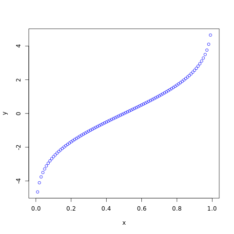
qnorm()

The qnorm() function takes the probability value and returns cumulative value corresponding to probability value of the distribution.

#creating a sequence of probability from
#0 to 1 with a difference of 0.01
x <- seq(0, 1, by=0.01)
   
y <- qnorm(x, 0, 2)
   
#naming the file
png(file = "normal.png")

#plotting the graph
plot(x, y, col="blue")

#saving the file
dev.off()

The output of the above code will be:

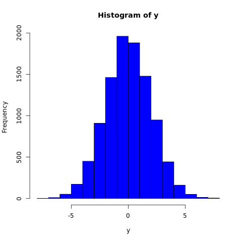
rnorm()

The rnorm() function generates a vector containing specified number of random values from the given normal distribution. In the example below, a histogram is plotted to visualize the result.

#fixing the seed to maintain the
#reproducibility of the result
set.seed(10)
x <- 10000

#creating a vector containing 10000
#normally distributed random values  
y <- rnorm(x, 0, 2)
   
#naming the file
png(file = "normal.png")

#plotting the graph
hist(y, col="blue")

#saving the file
dev.off()

The output of the above code will be: