R - Geometric Distribution
Geometric Distribution is a discrete probability distribution and it expresses the probability distribution of the random variable (X) representing number of failures before the first success.
The probability mass function (pmf) of geometric distribution is defined as:
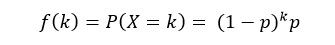
Where, k is the number of Bernoulli trials (k = 0,1,2...) and p is probability of success in each trial.
An geometric distribution has mean (1-p)/p and variance (1-p)/p2.
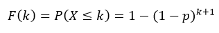
The cumulative distribution function (cdf) evaluated at k, is the probability that the random variable (X) will take a value less than or equal to k. The cdf of geometric distribution is defined as:
In R, there are four functions which can be used to generate geometric distribution.
Syntax
dgeom(x, prob)
pgeom(q, prob)
qgeom(p, prob)
rgeom(n, prob)
Parameters
x |
Required. Specify a vector of numbers. |
q |
Required. Specify a vector of numbers. |
p |
Required. Specify a vector of probabilities. |
n |
Required. Specify number of observation (sample size). |
prob |
Required. Specify probability of success in each trial. 0 < prob <= 1. |
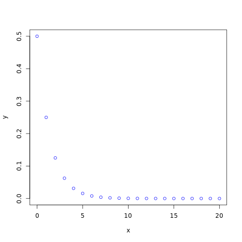
dgeom()
The dgeom() function measures probability mass function (pmf) of the distribution.
#creating a sequence of values between
#0 to 20 with a difference of 1
x <- seq(0, 20, by=1)

y <- dgeom(x, 0.5)

#naming the file
png(file = "geometric.png")

#plotting the graph
plot(x, y, col="blue")

#saving the file
dev.off()
The output of the above code will be:
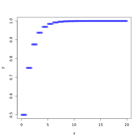
pgeom()
The pgeom() function returns cumulative distribution function (cdf) of the distribution.
#creating a sequence of values between
#0 to 20 with a difference of 0.1
x <- seq(0, 20, by=0.1)

y <- pgeom(x, 0.5)

#naming the file
png(file = "geometric.png")

#plotting the graph
plot(x, y, col="blue")

#saving the file
dev.off()
The output of the above code will be:
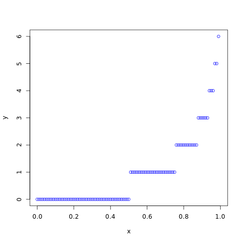
qgeom()
The qgeom() function takes the probability value and returns cumulative value corresponding to probability value of the distribution.
#creating a sequence of probability from
#0 to 1 with a difference of 0.01
x <- seq(0, 1, by=0.01)

y <- qgeom(x, 0.5)

#naming the file
png(file = "geometric.png")

#plotting the graph
plot(x, y, col="blue")

#saving the file
dev.off()
The output of the above code will be:
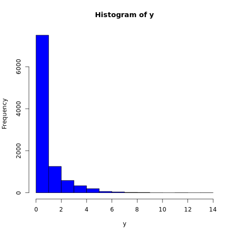
rgeom()
The rgeom() function generates a vector containing specified number of random values from the given geometric distribution. In the example below, a histogram is plotted to visualize the result.
#fixing the seed to maintain the
#reproducibility of the result
set.seed(10)
x <- 10000

#creating a vector containing 10000 random
#values from the given geometric distribution
y <- rgeom(x, 0.5)

#naming the file
png(file = "geometric.png")

#plotting the graph
hist(y, col="blue")

#saving the file
dev.off()
The output of the above code will be: