R - Histogram

A histogram is a graphical representation of the distribution of numerical data. To construct a histogram, the steps are given below:

Bin (or bucket) the range of values.
Divide the entire range of values into a series of intervals.
Count how many values fall into each interval.

The bins are usually specified as consecutive, non-overlapping intervals of a variable. The bins (intervals) must be adjacent and are often (but not required to be) of equal size.

The R hist() function computes and draws the histogram of the given data values.

Syntax

hist(x, freq, main, xlab, ylab, xlim, 
     ylim, col, border, breaks)

Parameters

`x`	`Required.` Specify a vector of values for which the histogram is desired.
`freq`	`Optional.` If TRUE, the histogram graphic is a representation of frequencies, the counts component of the result. If FALSE, probability densities, component density, are plotted.
`main, xlab, ylab`	`Optional.` Used to specify main title, x axis label and y axis label respectively.
`xlim, ylim`	`Optional.` Used to specify range of values on x-axis and y-axis respectively.
`col`	`Optional.` Specify a color to be used to fill the bars.
`border`	`Optional.` Specify the color of the border around the bars.
`breaks`	`Optional.` Used to specify the width of each bar. It can be one of the following: A vector giving the breakpoints between histogram cells. A function to compute the vector of breakpoints. A single number giving the number of cells for the histogram. A character string naming an algorithm to compute the number of cells. A function to compute the number of cells.

Example:

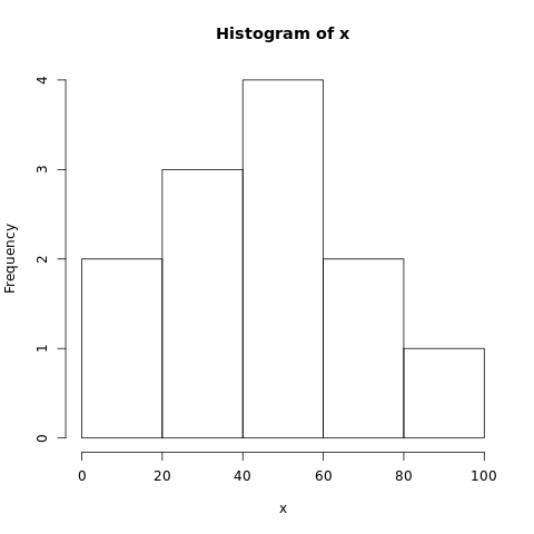
In the example below, a histogram is generated using data present in vector x.

#creating dataset
x <- c(45,64,5,22,55,89,59,35,78,42,34,15)

#naming the file
png(file = "histogram.png")

#drawing the histogram
hist(x)

#saving the file
dev.off()

The output of the above code will be:

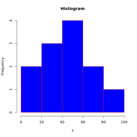
Example: Histogram title and color

More features in the plot can be added using more parameters in the function. To add title to the plot, main parameter is used and to add color, col parameter is used.

#creating dataset
x <- c(45,64,5,22,55,89,59,35,78,42,34,15)
#creating bins
bin <- c(0,20,40,60,80,100)

#naming the file
png(file = "histogram.png")

#drawing the histogram
hist(x, main='Histogram', col='blue', 
     border='red', breaks=bin)

#saving the file
dev.off()

The output of the above code will be:

Example: Probability density histogram

By specifying freq to FALSE, the histogram will represent probability densities instead of frequency. Please consider the example below.

#creating dataset
x <- c(45,64,5,22,55,89,59,35,78,42,34,15)
#creating bins
bin <- c(0,20,40,60,80,100)

#naming the file
png(file = "histogram.png")

#drawing the histogram
hist(x, main='Histogram', col='green', 
     border='red', breaks=bin, freq=FALSE)

#saving the file
dev.off()

The output of the above code will be:

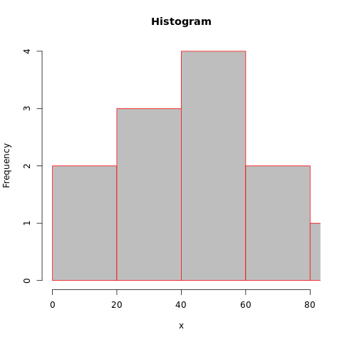
Example: Setting limits of data

By using xlim and ylim arguments, the histogram can be generated with a data in the specified range. In the example below, the data is limited to 80.

#creating dataset
x <- c(45,64,5,22,55,89,59,35,78,42,34,15)
#creating bins
bin <- c(0,20,40,60,80,100)

#naming the file
png(file = "histogram.png")

#drawing the histogram
hist(x, main='Histogram', col='grey', 
     border='red', breaks=bin, xlim=c(0,80) )

#saving the file
dev.off()

The output of the above code will be: