R - Uniform Distribution
Uniform Distribution describes an experiment where there is an random outcome that lies between certain bounds. The bounds of the outcome are defined by the parameters, a and b, which are the minimum and maximum values. All intervals of the same length on the distribution has equal probability.
The probability density function (pdf) of uniform distribution is defined as:
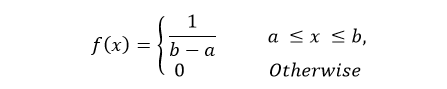
Where, a and b are lower and upper boundaries of output interval respectively.
An uniform distribution has mean (a+b)/2 and variance (b-a)2/12.
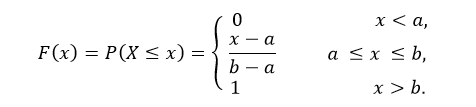
The cumulative distribution function (cdf) evaluated at x, is the probability that the random variable (X) will take a value less than or equal to x. The cdf of uniform distribution is defined as:
In R, there are four functions which can be used to generate uniform distribution.
Syntax
dunif(x, min, max)
punif(q, min, max)
qunif(p, min, max)
runif(n, min, max)
Parameters
x |
Required. Specify a vector of numbers. |
q |
Required. Specify a vector of numbers. |
p |
Required. Specify a vector of probabilities. |
n |
Required. Specify number of observation (sample size). |
min |
Optional. Specify lower limit of the distribution. Default is 0. |
max |
Optional. Specify upper limit of the distribution. Default is 1. |
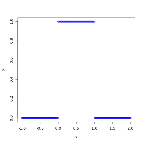
dunif()
The dunif() function measures probability density function (pdf) of the distribution.
#creating a sequence of values between
#-1 to 2 with a difference of 0.01
x <- seq(-1, 2, by=0.01)

y <- dunif(x, 0, 1)

#naming the file
png(file = "uniform.png")

#plotting the graph
plot(x, y, col="blue")

#saving the file
dev.off()
The output of the above code will be:
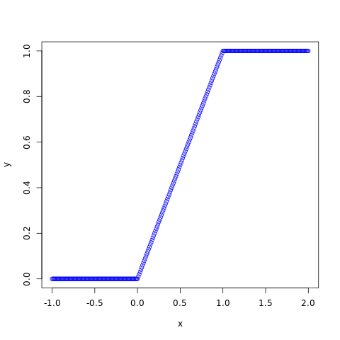
punif()
The punif() function returns cumulative distribution function (cdf) of the distribution.
#creating a sequence of values between
#-1 to 2 with a difference of 0.01
x <- seq(-1, 2, by=0.01)

y <- punif(x, 0, 1)

#naming the file
png(file = "uniform.png")

#plotting the graph
plot(x, y, col="blue")

#saving the file
dev.off()
The output of the above code will be:
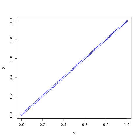
qunif()
The qunif() function takes the probability value and returns cumulative value corresponding to probability value of the distribution.
#creating a sequence of probability from
#0 to 1 with a difference of 0.01
x <- seq(0, 1, by=0.01)

y <- qunif(x, 0, 1)

#naming the file
png(file = "uniform.png")

#plotting the graph
plot(x, y, col="blue")

#saving the file
dev.off()
The output of the above code will be:
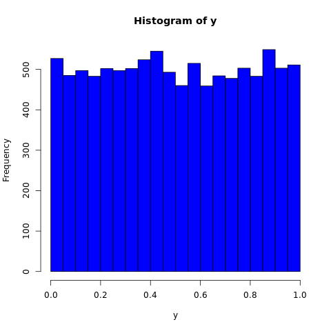
runif()
The runif() function generates a vector containing specified number of random values from the given uniform distribution. In the example below, a histogram is plotted to visualize the result.
#fixing the seed to maintain the
#reproducibility of the result
set.seed(10)
x <- 10000

#creating a vector containing 10000
#uniformly distributed random values
y <- runif(x, 0, 1)

#naming the file
png(file = "uniform.png")

#plotting the graph
hist(y, col="blue")

#saving the file
dev.off()
The output of the above code will be: