Matplotlib Tutorial

Matplotlib Tutorial

Matplotlib - Transformations

Like any graphics packages, Matplotlib is built on top of a transformation framework to easily move between coordinate systems, the userland data coordinate system, the axes coordinate system, the figure coordinate system, and the display coordinate system.

The table below summarizes the some useful coordinate systems, the transformation object in that coordinate system, and the description of that system. In the Transformation Object column, ax is a Axes instance, and fig is a Figure instance.

Coordinates	Transformation object	Description
"data"	ax.transData	The coordinate system for the data, controlled by xlim and ylim.
"axes"	ax.transAxes	The coordinate system of the Axes; (0, 0) is bottom left of the axes, and (1, 1) is top right of the axes.
"subfigure"	subfigure.transSubfigure	The coordinate system of the SubFigure; (0, 0) is bottom left of the subfigure, and (1, 1) is top right of the subfigure. If a figure has no subfigures, this is the same as transFigure.
"figure"	fig.transFigure	The coordinate system of the Figure; (0, 0) is bottom left of the figure, and (1, 1) is top right of the figure.
"figure-inches"	fig.dpi_scale_trans	The coordinate system of the Figure in inches; (0, 0) is bottom left of the figure, and (width, height) is the top right of the figure in inches.
"display"	None, or IdentityTransform()	The pixel coordinate system of the display window; (0, 0) is bottom left of the window, and (width, height) is top right of the display window in pixels.
"xaxis", "yaxis"	ax.get_xaxis_transform(), ax.get_yaxis_transform()	Blended coordinate systems; use data coordinates on one of the axis and axes coordinates on the other.

All of the transformation objects in the table above take inputs in their coordinate system, and transform the input to the display coordinate system.

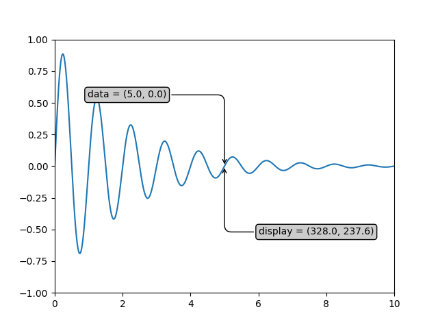
Example: data coordinates

In the example below, ax.transData instance is used to transform the data of a single to display coordinate system.

import matplotlib.pyplot as plt
import numpy as np

x = np.arange(0, 10, 0.005)
y = np.exp(-x/2.) * np.sin(2*np.pi*x)

fig, ax = plt.subplots()
ax.plot(x, y)
ax.set_xlim(0, 10)
ax.set_ylim(-1, 1)

xdata, ydata = 5, 0
#transforming the data to display coordinate system
xdisplay, ydisplay = ax.transData.transform((xdata, ydata))

bbox = dict(boxstyle="round", fc="0.8")
arrowprops = dict(
    arrowstyle="->",
    connectionstyle="angle,angleA=0,angleB=90,rad=10")

offset = 72
ax.annotate('data = (%.1f, %.1f)' % (xdata, ydata),
            (xdata, ydata), xytext=(-2*offset, offset), 
            textcoords='offset points',
            bbox=bbox, arrowprops=arrowprops)

disp = ax.annotate('display = (%.1f, %.1f)' % (xdisplay, ydisplay),
                   (xdisplay, ydisplay), xytext=(0.5*offset, -offset),
                   xycoords='figure pixels',
                   textcoords='offset points',
                   bbox=bbox, arrowprops=arrowprops)

plt.show()

The output of the above code will be:

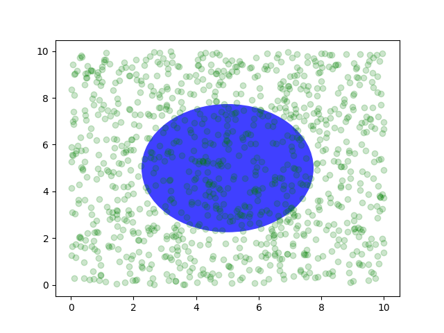
Python transforming data to display coordinate system

Example: axes coordinates

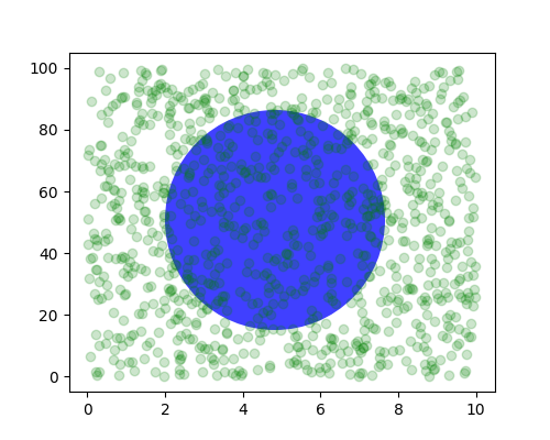
In the example below, plot of thousands random number in range 0 to 10 is plotted. Then, the ax.transAxes instance is used to overlay a semi-transparent circle centered in the middle of the axes with a radius one quarter of the axes. If the axes does not preserve aspect ratio, this will look like an ellipse (use: ax.set_aspect('equal').

import matplotlib.pyplot as plt
import numpy as np
import matplotlib.patches as mpatches

fig, ax = plt.subplots()
x, y = 10*np.random.rand(2, 1000)

#plot the data
ax.plot(x, y, 'go', alpha=0.2)

circ = mpatches.Circle((0.5, 0.5), 0.25, 
                       transform=ax.transAxes,
                       facecolor='blue', 
                       alpha=0.75)

ax.add_patch(circ)

plt.show()

The output of the above code will be:

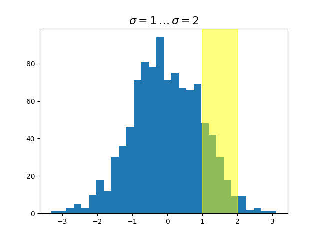
Python plot of thousands random number and an overlay of semi-transparent circle centered in the middle of the axes

Example: blended transformations

Drawing in blended coordinate spaces which mix axes with data coordinates is extremely useful. In the example below, a horizontal span is created which highlights some region of the y-data but spans across the x-axis regardless of the data limits, pan or zoom level, etc.

import matplotlib.pyplot as plt
import matplotlib.transforms as transforms
import matplotlib.patches as mpatches
import numpy as np

fig, ax = plt.subplots()
x = np.random.randn(1000)

ax.hist(x, 30)
ax.set_title(r'$\sigma=1 \/ \dots \/ \sigma=2$', fontsize=16)

#x coords of this transformation are data, 
#and the y coord are axes
trans = transforms.blended_transform_factory(
                ax.transData, ax.transAxes)

#highlight the 1-stddev to 2-stddev region with a span.
rect = mpatches.Rectangle((1, 0), width=1, height=1, 
                          transform=trans,
                          color='yellow', alpha=0.5)
ax.add_patch(rect)

plt.show()

The output of the above code will be:

Python creating blended transformation

Example: plotting in physical coordinates

Sometimes we want an object to be a certain physical size on the plot. In the example below, changing the size of the figure does not change the offset of the circle from the lower-left corner, does not change its size, and the circle remains a circle regardless of the aspect ratio of the axes.

import matplotlib.pyplot as plt
import numpy as np
import matplotlib.patches as mpatches

fig, ax = plt.subplots(figsize=(5, 4))
x, y = 10*np.random.rand(2, 1000)

#plot data
ax.plot(x, y*10., 'go', alpha=0.2)  

# add a circle in fixed-coordinates
circ = mpatches.Circle((2.5, 2), 1.0, 
                        transform=fig.dpi_scale_trans,
                        facecolor='blue', alpha=0.75)

ax.add_patch(circ)

plt.show()

The output of the above code will be:

Python Transformations

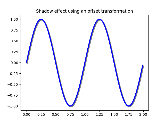
Example: using offset transforms to create a shadow effect

Another use of ScaledTranslation is to create a new transformation that is offset from another transformation, e.g., to place one object shifted a bit relative to another object.

One use for an offset is to create a shadow effect, where a object identical to the first is drawn just to the right of it, and just below it, adjusting the zorder to make sure the shadow is drawn first and then the object it is shadowing above it.

import matplotlib.pyplot as plt
import matplotlib.transforms as transforms
import matplotlib.patches as mpatches
import numpy as np

fig, ax = plt.subplots()

# make a simple sine wave
x = np.arange(0., 2., 0.01)
y = np.sin(2*np.pi*x)
line, = ax.plot(x, y, lw=3, color='blue')

# shift the object over 2 points, and down 2 points
dx, dy = 2/72., -2/72.
offset = transforms.ScaledTranslation(
           dx, dy, fig.dpi_scale_trans)
shadow_transform = ax.transData + offset

#plotting the same data with offset transform
#using the zorder to make it below the line
ax.plot(x, y, lw=3, color='gray',
        transform=shadow_transform,
        zorder=0.5*line.get_zorder())

ax.set_title('Shadow effect using an offset transformation')
plt.show()

The output of the above code will be:

Python using offset transforms to create a shadow effect

AlphaCodingSkills

AlphaCodingSkills Android App

AlphaCodingSkills is a online learning portal that provides tutorials on Python, Java, C++, C, C#, PHP, R, Ruby, Rust, Scala, Swift, Perl, SQL, Data Structures and Algorithms. Tutorials, examples, references and content of the website are reviewed and simplified continuously to improve comprehensibility and eliminate any possible error. We use cookies to ensure best browsing experience on our website. While using this website, you acknowledge to have read and accepted our cookie and privacy policy.